> ## Documentation Index
> Fetch the complete documentation index at: https://cubed3-igor-docs-funnel-chart.mintlify.site/llms.txt
> Use this file to discover all available pages before exploring further.
# Calculated fields
> Create ad-hoc custom dimensions and measures with Semantic SQL in workbooks, with help from AI or the field picker.
Calculated fields are ad-hoc dimensions and measures you add only to the current
workbook report. They do not change the shared data model.
As described in [Semantic SQL](/docs/introduction#semantic-sql), Cube routes
analysis through the semantic layer instead of sending arbitrary SQL straight to
the warehouse. The runtime validates every request and applies your security
policies. Semantic SQL builds on Postgres-compatible SQL—including the
`MEASURE()` function—so you can express derived logic on top of existing
semantic definitions with both flexibility and governance.
Calculated fields are expressed as Semantic SQL and pushed down to the Cube
backend for evaluation. The semantic layer compiles them with the rest of the
query—rather than applying them only in the browser—so the same validation,
governance, and warehouse execution path apply as for any other Semantic SQL
analysis.
## Using AI to create calculated fields
You can ask the Cube AI agent to create custom calculations in natural language.
The agent can add or refine calculated fields from different parts of the
product—for example while exploring in **Analytics chat** or working in
**Workbooks**—so you are not limited to a single entry point when you want a new
metric or dimension for the analysis in front of you.
## Creating calculated fields in UI
You can also build and edit calculated fields directly in the workbook. New
fields appear in the **Query fields** section of the field picker sidebar.
### Aggregations from existing dimensions
Right-click a dimension column header and choose an aggregation to create a
calculated field automatically. Available aggregations depend on the column type:
| Column type | Available aggregations |
| --------------- | -------------------------------------- |
| Number | Count Distinct, Sum, Average, Min, Max |
| Time | Count Distinct, Min, Max |
| String, Boolean | Count Distinct |
### Calculations from existing measures
Open the menu on a measure column header and use the **Calculations** submenu
for derived calculations:
| Calculation | Description |
| ---------------------- | ------------------------------------------------------- |
| % of total | Ratio of the measure value to the total across all rows |
| % of previous | Ratio of the measure value to the previous row's value |
| % change from previous | Percentage change compared to the previous row |
| Running total | Cumulative sum of the measure across rows |
**% of previous**, **% change from previous**, and **Running total** require at
least one dimension in the query.
Which calculations are offered depends on the measure’s aggregation type:
| Aggregation type | Available calculations |
| ----------------------- | ---------------------- |
| Count, Sum | All calculations |
| Min, Max | Running total |
| Average, Count Distinct | None |
### Filtered measures
When working with query **Results**, pivot so at least one dimension is on
columns, then open the header menu on a **pivoted measure column** and choose
**Create filtered measure**. Cube adds a calculated measure that applies the
column’s slice—for example, from **Count** broken down by **Status**, you get a
measure that only aggregates rows matching that status (such as completed
orders only).
The option appears only for **native** measures on pivoted columns, not for
calculated fields. The same flow works in **Explore** when results are pivoted
the same way.
### Bins and value groups
You can also bucket an existing dimension without writing SQL. Open its menu in
the field picker sidebar and choose **Create bins…** on a number dimension, or
**Group values…** on a string one. Time dimensions have granularities instead,
and an already derived field cannot be bucketed again.
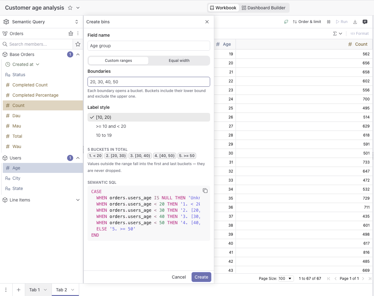 **Bins** take their boundaries either as a list (**Custom ranges**) or from a
**Start**, **Width**, and number of **Ranges** (**Equal width**). Each boundary
opens a bucket that includes its lower bound and excludes the upper one, and two
open-ended buckets are added at the edges—so `0, 18, 25` yields `< 0`, `[0, 18)`,
`[18, 25)`, `>= 25`, and no row is dropped. **Label style** renders a bucket as
`[10, 20)`, `>= 10 and < 20`, or `10 to 19`; the last is offered only while every
boundary is a whole number. Rows where the dimension is `NULL` are reported as
`Unknown`.
**Value groups** collect the dimension's values into named sets: pick values, name
the group, and choose **Add group**. A value belongs to one group at a time.
Whatever you did not pick—including empty values—falls under **Everything else**,
which defaults to `Other`.
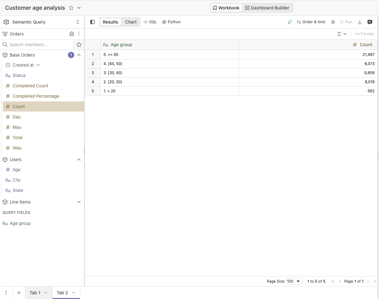
Bucket labels carry their position as a prefix (`1.`, `2.`, zero-padded past nine
buckets) so that sorting the column sorts it by value rather than alphabetically,
which would put `>= 25` before `[0, 18)`. The prefix is visible in results, chart
legends, and axes.
**Bins** take their boundaries either as a list (**Custom ranges**) or from a
**Start**, **Width**, and number of **Ranges** (**Equal width**). Each boundary
opens a bucket that includes its lower bound and excludes the upper one, and two
open-ended buckets are added at the edges—so `0, 18, 25` yields `< 0`, `[0, 18)`,
`[18, 25)`, `>= 25`, and no row is dropped. **Label style** renders a bucket as
`[10, 20)`, `>= 10 and < 20`, or `10 to 19`; the last is offered only while every
boundary is a whole number. Rows where the dimension is `NULL` are reported as
`Unknown`.
**Value groups** collect the dimension's values into named sets: pick values, name
the group, and choose **Add group**. A value belongs to one group at a time.
Whatever you did not pick—including empty values—falls under **Everything else**,
which defaults to `Other`.
Bucket labels carry their position as a prefix (`1.`, `2.`, zero-padded past nine
buckets) so that sorting the column sorts it by value rather than alphabetically,
which would put `>= 25` before `[0, 18)`. The prefix is visible in results, chart
legends, and axes.
 The panel previews the Semantic SQL it generates as you build:
```sql theme={null}
CASE WHEN orders_view.age IS NULL THEN 'Unknown'
WHEN orders_view.age < 0 THEN '1. < 0'
WHEN orders_view.age < 18 THEN '2. [0, 18)'
ELSE '3. >= 18' END
```
**Equal width** ranges are resolved into boundaries when the field is created, not
recomputed from the data. Values arriving later outside the range join the first
and last buckets instead of extending them.
To change a bucketed field, choose **Edit bins…** or **Edit groups…** from its
menu—either in the sidebar or on its column header in the results. Only fields
this panel generated offer the action; a `CASE` expression written by hand does
not.
### Editing a calculated field
Select a calculated field in the sidebar to open the editor. You can change its
**name** and **SQL expression**, then choose **Update** to apply.
The panel previews the Semantic SQL it generates as you build:
```sql theme={null}
CASE WHEN orders_view.age IS NULL THEN 'Unknown'
WHEN orders_view.age < 0 THEN '1. < 0'
WHEN orders_view.age < 18 THEN '2. [0, 18)'
ELSE '3. >= 18' END
```
**Equal width** ranges are resolved into boundaries when the field is created, not
recomputed from the data. Values arriving later outside the range join the first
and last buckets instead of extending them.
To change a bucketed field, choose **Edit bins…** or **Edit groups…** from its
menu—either in the sidebar or on its column header in the results. Only fields
this panel generated offer the action; a `CASE` expression written by hand does
not.
### Editing a calculated field
Select a calculated field in the sidebar to open the editor. You can change its
**name** and **SQL expression**, then choose **Update** to apply.